On the use of the Kullback–Leibler divergence in Variational Autoencoders

可變自動編碼器(VAE)的loss function可以分為兩部分。第一個測量autoencoding的量，即原始樣本與其重構之間的誤差。第二個是有關standard multivariate normal distribution的Kullback-Leibler散度(縮寫為KL散度)。我們將畫圖說明KL散度對encoder 和decoder 輸出的影響。



loss function中KL發散項的目的是使encoder輸出的分佈盡可能接近standard multivariate normal distribution。接下來，我們將考慮一個latent space為2的autoencoder 。我們首先在二維情況下繪製standard multivariate normal distribution的樣本點。

%matplotlib inline
import numpy as np
import matplotlib.pyplot as plt

plt.figure(figsize=(12, 10))
z = np.random.multivariate_normal([0] * 2, np.eye(2), 5000)
plt.scatter(z[:, 0], z[:, 1])
plt.xlabel("z[0]")
plt.ylabel("z[1]")
plt.title('Samples from a 2D standard multivariate normal distribution')
plt.show()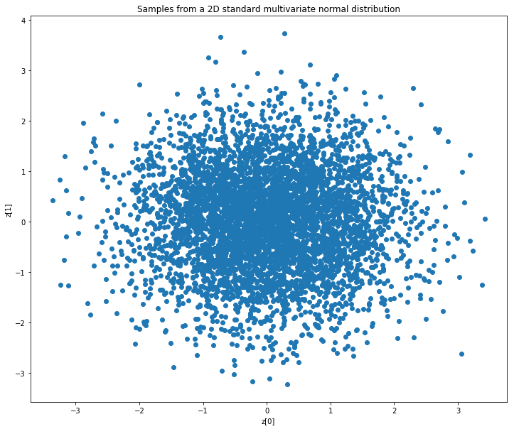

encoder的理想輸出看起來與上面的圖類似。

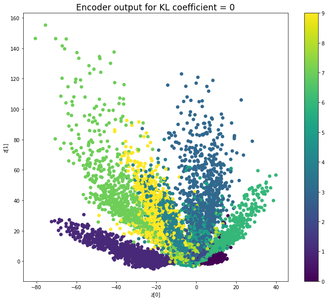
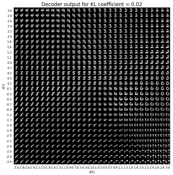
接下來，我們將修改Keras範例中的Variational Autoencoder，以顯示KL散度如何影響encoder和decoder輸出。 我們將係數c添加到KL散度。 因此，損失函數變為loss = reconstruction_loss + c * kl_loss。 我們看一下不同的c值所呈現出來的結果。

'''Example showing the influence of the KL divergence on the encoder and 
decoder ouputs.

This is a modification of Keras VAE example that is available at:
https://github.com/keras-team/keras/blob/master/examples/variational_autoencoder.py
'''

from keras.layers import Lambda, Input, Dense
from keras.models import Model
from keras.datasets import mnist
from keras.losses import binary_crossentropy
from keras.optimizers import Adam
from keras import backend as K

import numpy as np
import matplotlib.pyplot as plt
from tqdm import tqdm

# reparameterization trick
# instead of sampling from Q(z|X), sample epsilon = N(0,I)
# z = z_mean + sqrt(var) * epsilon
def sampling(args):
    """Reparameterization trick by sampling from an isotropic unit Gaussian.
    # Arguments
        args (tensor): mean and log of variance of Q(z|X)
    # Returns
        z (tensor): sampled latent vector
    """

    z_mean, z_log_var = args
    batch = K.shape(z_mean)[0]
    dim = K.int_shape(z_mean)[1]
    # by default, random_normal has mean = 0 and std = 1.0
    epsilon = K.random_normal(shape=(batch, dim))
    return z_mean + K.exp(0.5 * z_log_var) * epsilon


def plot_results(models,
                 data,
                 kl_coefficient,
                 batch_size=128):
    """Plots labels and MNIST digits as a function of the 2D latent vector
    # Arguments
        models (tuple): encoder and decoder models
        data (tuple): test data and label
        batch_size (int): prediction batch size
        kl_coefficient (double): the KL loss coefficient 
    """

    encoder, decoder = models
    x_test, y_test = data

    # display a 2D plot of the digit classes in the latent space
    z_mean, _, _ = encoder.predict(x_test,
                                   batch_size=batch_size)
    plt.figure(figsize=(12, 10))
    plt.scatter(z_mean[:, 0], z_mean[:, 1], c=y_test)
    plt.colorbar()
    plt.xlabel("z[0]")
    plt.ylabel("z[1]")
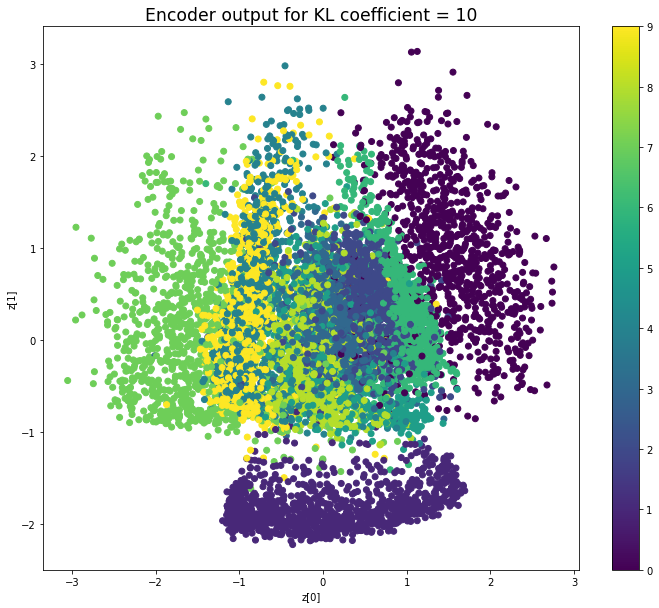
    plt.title(f'Encoder output for KL coefficient = {kl_coefficient}', fontdict={'fontsize': 'xx-large'})
    plt.show()

    print('\n')
    
    # display a 30x30 2D manifold of digits
    n = 30
    digit_size = 28
    figure = np.zeros((digit_size * n, digit_size * n))
    # linearly spaced coordinates corresponding to the 2D plot
    # of digit classes in the latent space
    grid_x = np.linspace(-3, 3, n)
    grid_y = np.linspace(-3, 3, n)[::-1]

    for i, yi in enumerate(grid_y):
        for j, xi in enumerate(grid_x):
            z_sample = np.array([[xi, yi]])
            x_decoded = decoder.predict(z_sample)
            digit = x_decoded[0].reshape(digit_size, digit_size)
            figure[i * digit_size: (i + 1) * digit_size,
                   j * digit_size: (j + 1) * digit_size] = digit

    plt.figure(figsize=(10, 10))
    start_range = digit_size // 2
    end_range = (n - 1) * digit_size + start_range + 1
    pixel_range = np.arange(start_range, end_range, digit_size)
    sample_range_x = np.round(grid_x, 1)
    sample_range_y = np.round(grid_y, 1)
    plt.xticks(pixel_range, sample_range_x)
    plt.yticks(pixel_range, sample_range_y)
    plt.xlabel("z[0]")
    plt.ylabel("z[1]")
    plt.imshow(figure, cmap='Greys_r')
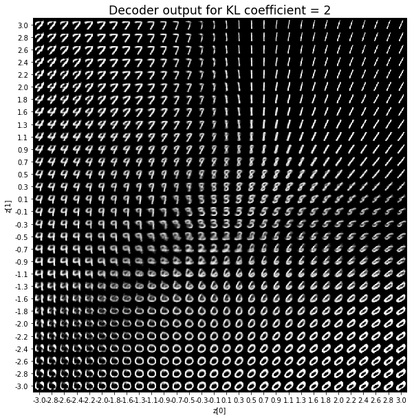
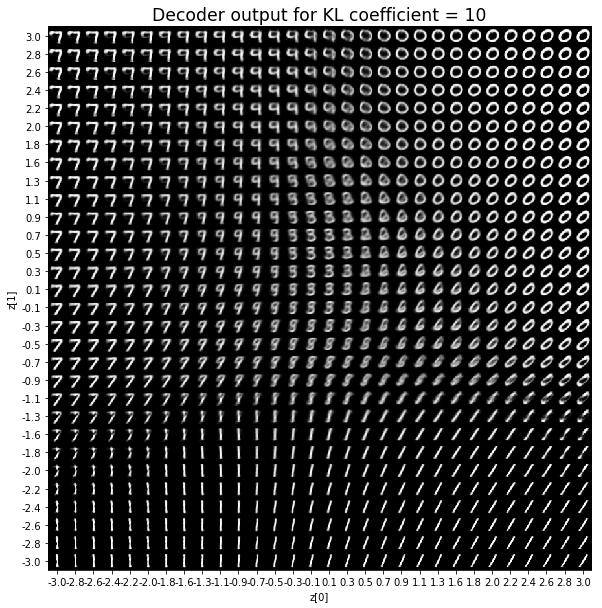
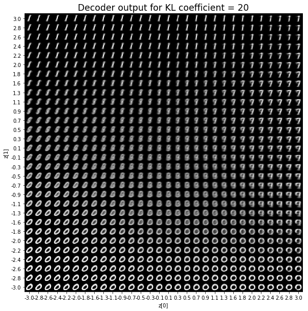
    plt.title(f'Decoder output for KL coefficient = {kl_coefficient}', fontdict={'fontsize': 'xx-large'})
    plt.show()

    
def build_model(input_shape, intermediate_dim, latent_dim, original_dim):
    # VAE model = encoder + decoder
    # build encoder model
    inputs = Input(shape=input_shape, name='encoder_input')
    x = Dense(intermediate_dim, activation='relu')(inputs)
    z_mean = Dense(latent_dim, name='z_mean')(x)
    z_log_var = Dense(latent_dim, name='z_log_var')(x)

    # use reparameterization trick to push the sampling out as input
    # note that "output_shape" isn't necessary with the TensorFlow backend
    z = Lambda(sampling, output_shape=(latent_dim,), name='z')([z_mean, z_log_var])

    # instantiate encoder model
    encoder = Model(inputs, [z_mean, z_log_var, z], name='encoder')

    # build decoder model
    latent_inputs = Input(shape=(latent_dim,), name='z_sampling')
    x = Dense(intermediate_dim, activation='relu')(latent_inputs)
    outputs = Dense(original_dim, activation='sigmoid')(x)

    # instantiate decoder model
    decoder = Model(latent_inputs, outputs, name='decoder')

    # instantiate VAE model
    outputs = decoder(encoder(inputs)[2])
    vae = Model(inputs, outputs, name='vae_mlp')

    models = (encoder, decoder)

    reconstruction_loss = binary_crossentropy(inputs, outputs)
    reconstruction_loss *= original_dim
    reconstruction_loss = K.mean(reconstruction_loss)

    kl_loss = 1 + z_log_var - K.square(z_mean) - K.exp(z_log_var)
    kl_loss = K.sum(kl_loss, axis=-1)
    kl_loss *= -0.5
    kl_loss = K.mean(kl_loss)
    
    return vae, models, reconstruction_loss, kl_loss
    
    
# MNIST dataset
(x_train, y_train), (x_test, y_test) = mnist.load_data()

image_size = x_train.shape[1]
original_dim = image_size * image_size
x_train = np.reshape(x_train, [-1, original_dim])
x_test = np.reshape(x_test, [-1, original_dim])
x_train = x_train.astype('float32') / 255
x_test = x_test.astype('float32') / 255

# network parameters
input_shape = (original_dim, )
intermediate_dim = 512
batch_size = 128
latent_dim = 2
epochs = 40

data = (x_test, y_test)

vae, _, _, _ = build_model(input_shape, intermediate_dim, latent_dim, original_dim)
vae.save_weights('vae_init.h5')

for kl_coefficient in [0, 0.02, 0.1, 0.5, 1, 2, 10, 20]:
    print('—' * 80)
    print('KL coefficient:', kl_coefficient, flush=True)
    vae, models, reconstruction_loss, kl_loss = build_model(input_shape, intermediate_dim, latent_dim, original_dim)
    vae.load_weights('vae_init.h5')
    vae_loss = reconstruction_loss + kl_coefficient * kl_loss
    vae.add_loss(vae_loss)
    vae.compile(optimizer=Adam(lr=1e-3))
    vae.metrics_tensors.append(reconstruction_loss)
    vae.metrics_name

KL coefficient: 0





KL coefficient: 0.02





KL coefficient: 0.1






KL coefficient: 0.5






KL coefficient: 1






KL coefficient: 2






KL coefficient: 10





KL coefficient: 20






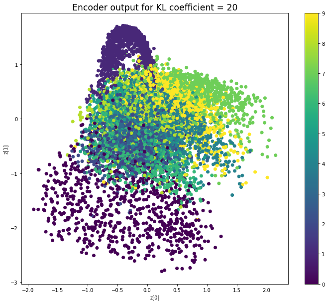
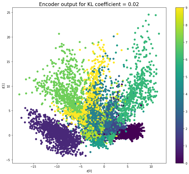
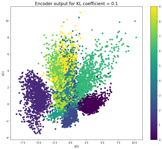
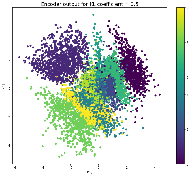
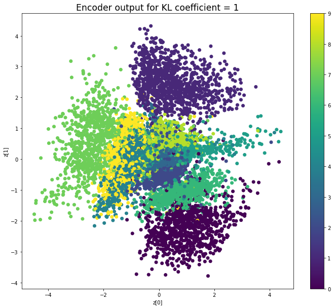
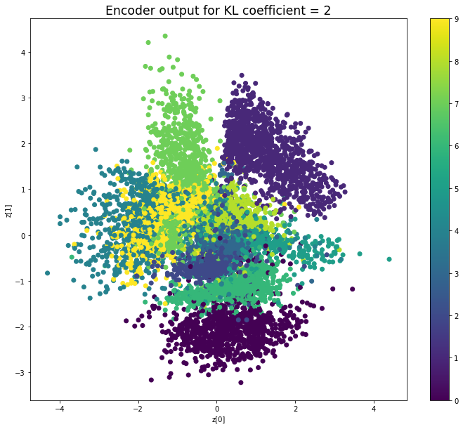
當不使用KL loss (係數= 0)時，encoder 的輸出值實際上是分散的。 增加係數時，值開始在原點附近聚集。 雖然遠非完美，但我們看到正確選擇的係數有助於使結果更接近2D standard multivariate normal distribution的參考圖。


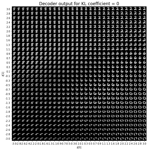
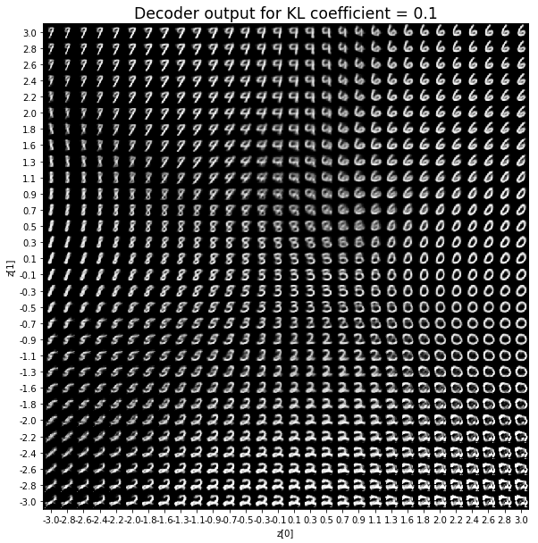
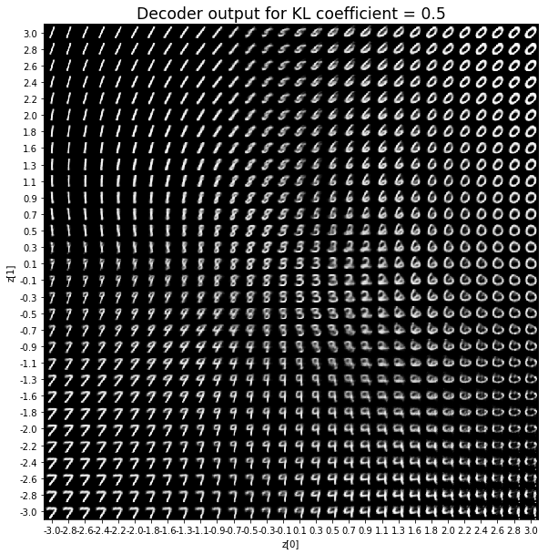
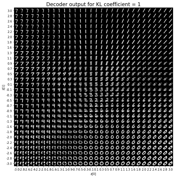
對於解碼器輸出，係數越大，結果得到的模糊值越多，數字越少。 很小的係數似乎也無法生成所有數字。總體而言，平均係數(例如0.5、1和2)似乎提供了最佳結果。

在前面的範例中，為reconstruction loss和KL loss選擇相等的權重可獲得良好的結果。 但是，請小心，這可能取決於所研究的問題以及如何定義損失。 例如，上述reconstruction loss被定義為image_dim * binary_crossentropy，而不是binary_crossentropy。



參考
https://www.vincent-lunot.com/post/on-the-use-of-the-kullback-leibler-divergence-in-variational-autoencoders/