2019年7月31日 星期三

2019年7月30日 星期二
Visualizing intermediate activation in Convolutional Neural Networks with Keras
在本文中,我們將使用Keras和Python訓練一個簡單的捲積神經網絡,用於分類任務。為此我們將使用一個非常小而簡單的圖像集,其中包括100張圓形圖畫,100張正方形圖片和100張三角形圖片,我在Kaggle中找到了這些圖片。這些將被分成訓練和測試集並饋送到網絡。
最重要的是,我們將在FrançoisChollet的“使用Python深度學習”書中複製一些工作,以便了解我們的層結構如何根據每個中間激活的可視化處理數據,其中包括顯示由網絡中的捲積和池化層輸出的feature maps。
這意味著我們將可視化每個激活層的結果。
我們將快速倒ㄌ,因為我們沒有專注於使用Keras解釋CNN的細節。
我們先導入所有必需的函式庫:
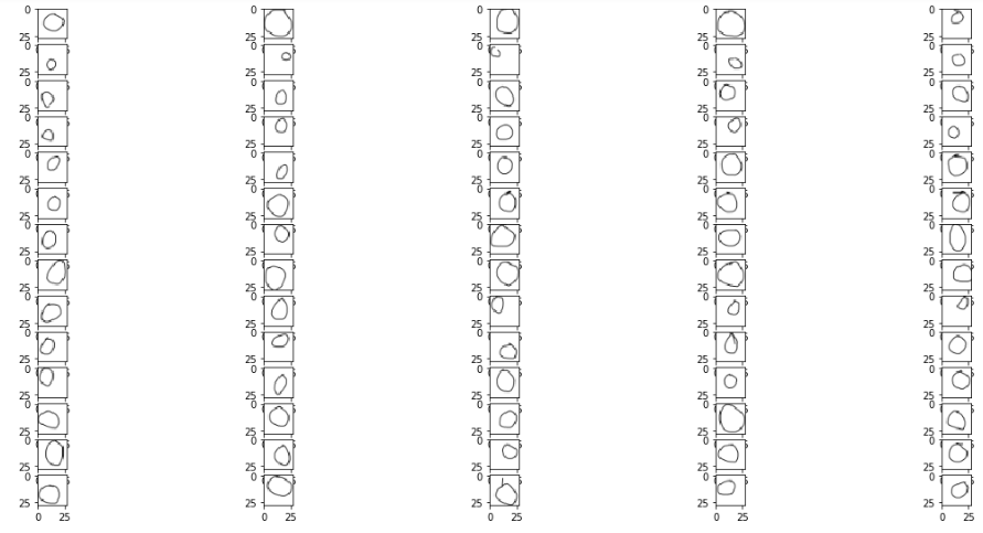
這些是我們的訓練圖像:
Circles
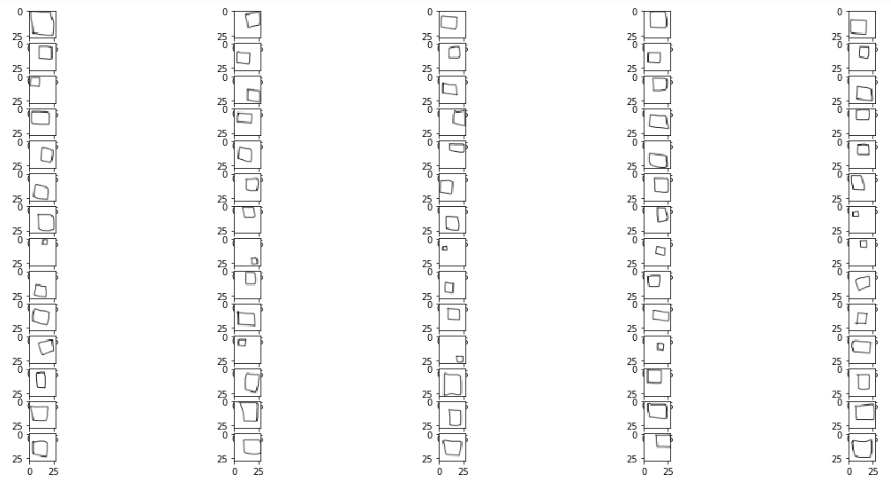
正方形
(代碼與上面幾乎相同,請在此處查看完整代碼)
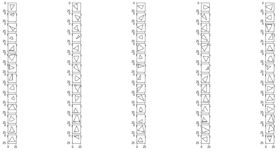
Triangles
圖像形狀在RGB比例中為28像素乘28像素(儘管它們僅可以說是黑色和白色)。
現在讓我們繼續我們的捲積神經網絡構造。 通常,我們使用Sequential()啟動模型:
我們指定卷積層並將MaxPooling添加到降低取樣和Dropout以防止過度擬合。 我們使用Flatten並以3個單位的密集層結束,每個類別(circle [0],square [1],triangle [1])。 我們將softmax指定為我們的最後一個激活函數,建議用於多類分類。
對於這種類型的圖像,一旦我們看一下這些feature maps就會很明顯了解我可能正在構建一個過於複雜的結構,但是它可以幫助我準確地展示每個層的內容。不過我確信我們可以用更少的層和更少的複雜性獲得相同或更好的結果。
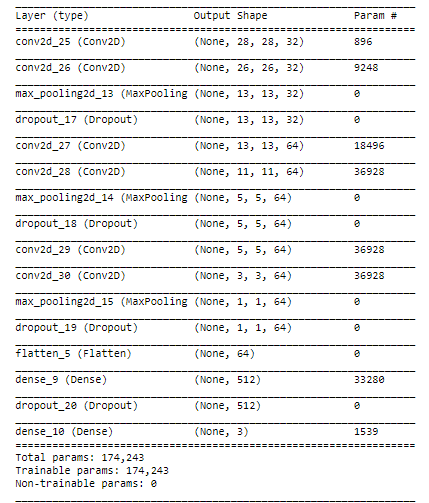
來看看我們的模型摘要:
我們使用rmsprop作為我們的優化器編譯模型,使用categorical_crossentropy作為我們的損失函數,並將accuracy指定為metric:
此時我們需要將圖片轉換為模型可以接受的形狀。 為此,我們使用ImageDataGenerator。 我們啟動它並使用.flow_from_directory提供圖像。 工作目錄中有兩個主文件夾,名為training_set和test_set。 每個子文件夾都有3個子文件夾,分別稱為circles,squares和triangles。 我已經將每個形狀的70個圖像發送到training_set,將30個圖像發送到test_set。
該模型將訓練30個epochs,但我們將使用ModelCheckpoint來存儲表現最佳epoch的權重。 我們將val_acc指定為用於定義最佳模型的metric。 這意味著我們將保持在測試集上的準確度方面得分最高的epoch的權重。
Training the model
現在是時候訓練模型了,這裡我們包括對checkpointer的callback
該模型訓練了20個epochs,並在epochs 10達到了它的最佳表現。我們得到以下資訊:
`Epoch 00010:val_acc從0.93333提高到0.95556,將模型保存到best_weights.hdf5`
在那之後,模型沒有針對下一個epochs進行改進,因此epochs 10的權重是被存儲的 - 這意味著我們現在有一個hdf5文件存儲該特定epoch的權重,其中測試集的準確度為95.6%
我們將確保我們的分類器加載了最佳權重
最後,讓我們保存最終模型以供日後使用:
Displaying curves of loss and accuracy during training
現在讓我們來看看我們的模型在30個epochs中的表現:
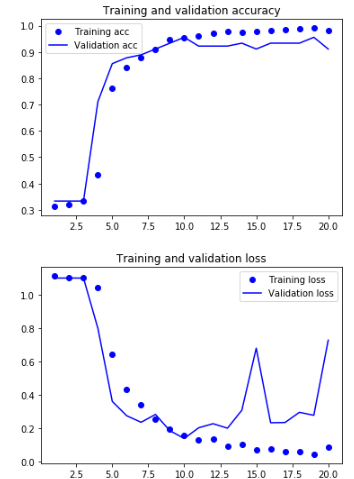
我們可以看到,在第10個epoch之後,模型開始過度擬合。 無論如何,我們保留了具有最佳性能的epoch結果。
Classes
讓我們現在闡明分配給我們每個圖片集的類別編號,因為這就是模型將如何產生它的預測:
circles:0
squres:1
triangles:2
Predicting the class of unseen images
藉由我們的模型訓練和存儲,我們可以從我們的測試集中加載一個簡單的未見過的圖像,看看它是如何分類的:
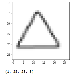
預測是類別[2],它是一個三角形。
到現在為止還挺好。 我們現在進入本文最重要的部分
Visualizing intermediate activations
引用FrançoisChollet的書“DEEP LEARNING with Python”(我將在本節中引用他很多):
中間激活“有助於理解連續的convnet層如何轉換其輸入,以及首先了解各個convnet濾波器的含義。”
“通過網絡學習所獲得的表徵(representations)非常適合可視化,這在很大程度上是因為它們是視覺概念的表現形式。可視化中間激活包括在給定特定輸入的情況下顯示由網絡中的各種卷積和池化層輸出的feature maps(層的輸出通常稱為其激活,激活函數的輸出)。這給出瞭如何藉由網絡學習將輸入分解成不同過濾器。每個通道編碼相對獨立的特徵,因此可視化這些feature maps的正確方法是將每個通道的內容獨立繪製為2D圖像。
接下來,我們將得到一個輸入圖像 - 一個三角形的圖片,而不是網絡訓練過的圖像的一部分。
“為了提取我們想要查看的feature maps,我們將創建一個Keras模型,該模型將批量圖像作為輸入,並輸出所有捲積和池化層的激活。為此,我們將使用Keras類別Model。使用兩個參數來實例化模型:輸入張量(或輸入張量list)和輸出張量(或輸出張量list)。結果類別是Keras模型,就像Sequential模型一樣,將指定的輸入映射到指定的輸出。 Model類別與眾不同之處在於,與Sequential不同,它允許具有多個輸出的模型。“
Instantiating a model from an input tensor and a list of output tensors
當輸入圖像輸入時,此模型返回原始模型中圖層激活的值。
For instance, this is the activation of the first convolution layer for the image input:
它是一個28×28的feature map,有32個通道。 讓我們嘗試繪製原始模型第一層激活的第四個通道
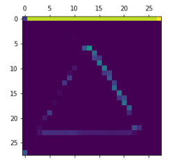
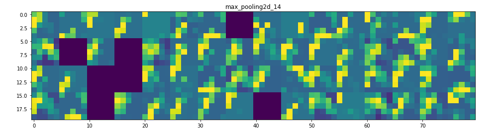
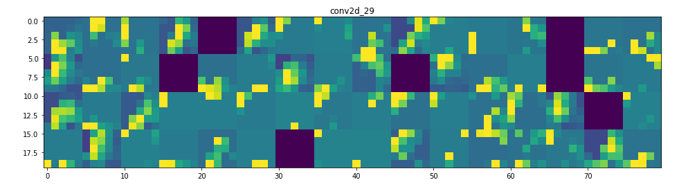
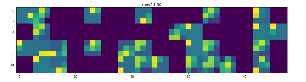
甚至在我們嘗試解釋這種激活之前,讓我們在每一層上繪製同一圖像的所有激活
Visualizing every channel in every intermediate activation
可在此處找到此部分的完整代碼
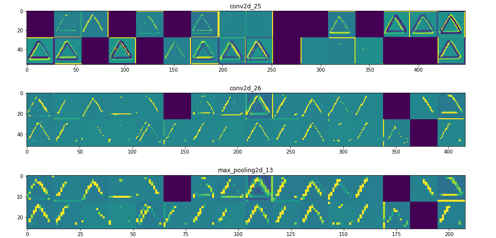
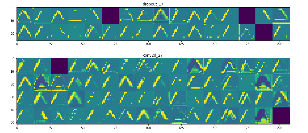

所以在這裡!讓我們試著解釋發生了什麼:
1. 第一層可以保留triangle的完整形狀,儘管有幾個過濾器未被激活並留空。在那個階段,激活幾乎保留了初始圖片中的所有資訊。
2. 隨著我們在各個層面的深入,激活變得越來越抽象,在視覺上也不那麼容易理解。他們開始編碼更高級別的概念,如單邊框,角落和角度。較高的presentations帶來關於圖像的視覺內容的資訊越來越少,並且越來越多的資訊與圖像的類別相關。
3. 如上所述,模型結構過於復雜,我們可以看到我們的最後一層實際上根本沒有激活,在那一點上沒有什麼需要學習的。
這就是它!我們已經可視化卷積神經網絡如何在一些基本圖形中找到模式以及它如何將資訊從一個層傳遞到另一個層。
參考
https://towardsdatascience.com/visualizing-intermediate-activation-in-convolutional-neural-networks-with-keras-260b36d60d0?fbclid=IwAR2GqxH-5EwqPycPVy-IhliMQKesA3gJMwJltWishQuv8c9rxzCIKPIa5sQ
最重要的是,我們將在FrançoisChollet的“使用Python深度學習”書中複製一些工作,以便了解我們的層結構如何根據每個中間激活的可視化處理數據,其中包括顯示由網絡中的捲積和池化層輸出的feature maps。
這意味著我們將可視化每個激活層的結果。
我們將快速倒ㄌ,因為我們沒有專注於使用Keras解釋CNN的細節。
我們先導入所有必需的函式庫:
%matplotlib inline
import glob
import matplotlib
from matplotlib import pyplot as plt
import matplotlib.image as mpimg
import numpy as np
import imageio as im
from keras import models
from keras.models import Sequential
from keras.layers import Conv2D
from keras.layers import MaxPooling2D
from keras.layers import Flatten
from keras.layers import Dense
from keras.layers import Dropout
from keras.preprocessing import image
from keras.preprocessing.image import ImageDataGenerator
from keras.callbacks import ModelCheckpoint
這些是我們的訓練圖像:
Circles
images = []
for img_path in glob.glob('training_set/circles/*.png'):
    images.append(mpimg.imread(img_path))
plt.figure(figsize=(20,10))
columns = 5
for i, image in enumerate(images):
    plt.subplot(len(images) / columns + 1, columns, i + 1)
    plt.imshow(image)
正方形
(代碼與上面幾乎相同,請在此處查看完整代碼)
Triangles
圖像形狀在RGB比例中為28像素乘28像素(儘管它們僅可以說是黑色和白色)。
現在讓我們繼續我們的捲積神經網絡構造。 通常,我們使用Sequential()啟動模型:
# Initialising the CNN
classifier = Sequential()
我們指定卷積層並將MaxPooling添加到降低取樣和Dropout以防止過度擬合。 我們使用Flatten並以3個單位的密集層結束,每個類別(circle [0],square [1],triangle [1])。 我們將softmax指定為我們的最後一個激活函數,建議用於多類分類。
# Step 1 - Convolution
classifier.add(Conv2D(32, (3, 3), padding='same', input_shape = (28, 28, 3), activation = 'relu'))
classifier.add(Conv2D(32, (3, 3), activation='relu'))
classifier.add(MaxPooling2D(pool_size=(2, 2)))
classifier.add(Dropout(0.5)) # antes era 0.25
# Adding a second convolutional layer
classifier.add(Conv2D(64, (3, 3), padding='same', activation = 'relu'))
classifier.add(Conv2D(64, (3, 3), activation='relu'))
classifier.add(MaxPooling2D(pool_size=(2, 2)))
classifier.add(Dropout(0.5)) # antes era 0.25
# Adding a third convolutional layer
classifier.add(Conv2D(64, (3, 3), padding='same', activation = 'relu'))
classifier.add(Conv2D(64, (3, 3), activation='relu'))
classifier.add(MaxPooling2D(pool_size=(2, 2)))
classifier.add(Dropout(0.5)) # antes era 0.25
# Step 3 - Flattening
classifier.add(Flatten())
# Step 4 - Full connection
classifier.add(Dense(units = 512, activation = 'relu'))
classifier.add(Dropout(0.5))
classifier.add(Dense(units = 3, activation = 'softmax'))
對於這種類型的圖像,一旦我們看一下這些feature maps就會很明顯了解我可能正在構建一個過於複雜的結構,但是它可以幫助我準確地展示每個層的內容。不過我確信我們可以用更少的層和更少的複雜性獲得相同或更好的結果。
來看看我們的模型摘要:
classifier.summary()
我們使用rmsprop作為我們的優化器編譯模型,使用categorical_crossentropy作為我們的損失函數,並將accuracy指定為metric:
# Compiling the CNN
classifier.compile(optimizer = 'rmsprop',
                   loss = 'categorical_crossentropy',
                   metrics = ['accuracy'])
此時我們需要將圖片轉換為模型可以接受的形狀。 為此,我們使用ImageDataGenerator。 我們啟動它並使用.flow_from_directory提供圖像。 工作目錄中有兩個主文件夾,名為training_set和test_set。 每個子文件夾都有3個子文件夾,分別稱為circles,squares和triangles。 我已經將每個形狀的70個圖像發送到training_set,將30個圖像發送到test_set。
train_datagen = ImageDataGenerator(rescale = 1./255)
test_datagen = ImageDataGenerator(rescale = 1./255)
training_set = train_datagen.flow_from_directory('training_set',target_size = (28,28), batch_size = 16, class_mode = 'categorical')
test_set = test_datagen.flow_from_directory('test_set',
                                            target_size = (28, 28), batch_size = 16, class_mode = 'categorical')
該模型將訓練30個epochs,但我們將使用ModelCheckpoint來存儲表現最佳epoch的權重。 我們將val_acc指定為用於定義最佳模型的metric。 這意味著我們將保持在測試集上的準確度方面得分最高的epoch的權重。
checkpointer = ModelCheckpoint(filepath="best_weights.hdf5",
                               monitor = 'val_acc',
                               verbose=1,
                               save_best_only=True)
Training the model
現在是時候訓練模型了,這裡我們包括對checkpointer的callback
history = classifier.fit_generator(training_set,
                                   steps_per_epoch = 100,
                                   epochs = 20,
                                   callbacks=[checkpointer],
                                   validation_data = test_set,
                                   validation_steps = 50)
該模型訓練了20個epochs,並在epochs 10達到了它的最佳表現。我們得到以下資訊:
`Epoch 00010:val_acc從0.93333提高到0.95556,將模型保存到best_weights.hdf5`
在那之後,模型沒有針對下一個epochs進行改進,因此epochs 10的權重是被存儲的 - 這意味著我們現在有一個hdf5文件存儲該特定epoch的權重,其中測試集的準確度為95.6%
我們將確保我們的分類器加載了最佳權重
classifier.load_weights('best_weights.hdf5')
最後,讓我們保存最終模型以供日後使用:
classifier.save('shapes_cnn.h5')
Displaying curves of loss and accuracy during training
現在讓我們來看看我們的模型在30個epochs中的表現:
acc = history.history['acc']
val_acc = history.history['val_acc']
loss = history.history['loss']
val_loss = history.history['val_loss']
epochs = range(1, len(acc) + 1)
plt.plot(epochs, acc, 'bo', label='Training acc')
plt.plot(epochs, val_acc, 'b', label='Validation acc')
plt.title('Training and validation accuracy')
plt.legend()
plt.figure()
plt.plot(epochs, loss, 'bo', label='Training loss')
plt.plot(epochs, val_loss, 'b', label='Validation loss')
plt.title('Training and validation loss')
plt.legend()
plt.show()
我們可以看到,在第10個epoch之後,模型開始過度擬合。 無論如何,我們保留了具有最佳性能的epoch結果。
Classes
讓我們現在闡明分配給我們每個圖片集的類別編號,因為這就是模型將如何產生它的預測:
circles:0
squres:1
triangles:2
Predicting the class of unseen images
藉由我們的模型訓練和存儲,我們可以從我們的測試集中加載一個簡單的未見過的圖像,看看它是如何分類的:
img_path = 'test_set/triangles/drawing(2).png'
img = image.load_img(img_path, target_size=(28, 28))
img_tensor = image.img_to_array(img)
img_tensor = np.expand_dims(img_tensor, axis=0)
img_tensor /= 255.
plt.imshow(img_tensor[0])
plt.show()
print(img_tensor.shape)
# predicting images
x = image.img_to_array(img)
x = np.expand_dims(x, axis=0)
images = np.vstack([x])
classes = classifier.predict_classes(images, batch_size=10)
print("Predicted class is:",classes)
> Predicted class is: [2]
預測是類別[2],它是一個三角形。
到現在為止還挺好。 我們現在進入本文最重要的部分
Visualizing intermediate activations
引用FrançoisChollet的書“DEEP LEARNING with Python”(我將在本節中引用他很多):
中間激活“有助於理解連續的convnet層如何轉換其輸入,以及首先了解各個convnet濾波器的含義。”
“通過網絡學習所獲得的表徵(representations)非常適合可視化,這在很大程度上是因為它們是視覺概念的表現形式。可視化中間激活包括在給定特定輸入的情況下顯示由網絡中的各種卷積和池化層輸出的feature maps(層的輸出通常稱為其激活,激活函數的輸出)。這給出瞭如何藉由網絡學習將輸入分解成不同過濾器。每個通道編碼相對獨立的特徵,因此可視化這些feature maps的正確方法是將每個通道的內容獨立繪製為2D圖像。
接下來,我們將得到一個輸入圖像 - 一個三角形的圖片,而不是網絡訓練過的圖像的一部分。
“為了提取我們想要查看的feature maps,我們將創建一個Keras模型,該模型將批量圖像作為輸入,並輸出所有捲積和池化層的激活。為此,我們將使用Keras類別Model。使用兩個參數來實例化模型:輸入張量(或輸入張量list)和輸出張量(或輸出張量list)。結果類別是Keras模型,就像Sequential模型一樣,將指定的輸入映射到指定的輸出。 Model類別與眾不同之處在於,與Sequential不同,它允許具有多個輸出的模型。“
Instantiating a model from an input tensor and a list of output tensors
layer_outputs = [layer.output for layer in classifier.layers[:12]]
# Extracts the outputs of the top 12 layers
activation_model = models.Model(inputs=classifier.input, outputs=layer_outputs) # Creates a model that will return these outputs, given the model input
當輸入圖像輸入時,此模型返回原始模型中圖層激活的值。
Running the model in predict mode
activations = activation_model.predict(img_tensor)
# Returns a list of five Numpy arrays: one array per layer activation
For instance, this is the activation of the first convolution layer for the image input:
first_layer_activation = activations[0]
print(first_layer_activation.shape)
(1, 28, 28, 32)
它是一個28×28的feature map,有32個通道。 讓我們嘗試繪製原始模型第一層激活的第四個通道
plt.matshow(first_layer_activation[0, :, :, 4], cmap='viridis')
甚至在我們嘗試解釋這種激活之前,讓我們在每一層上繪製同一圖像的所有激活
Visualizing every channel in every intermediate activation
可在此處找到此部分的完整代碼
所以在這裡!讓我們試著解釋發生了什麼:
1. 第一層可以保留triangle的完整形狀,儘管有幾個過濾器未被激活並留空。在那個階段,激活幾乎保留了初始圖片中的所有資訊。
2. 隨著我們在各個層面的深入,激活變得越來越抽象,在視覺上也不那麼容易理解。他們開始編碼更高級別的概念,如單邊框,角落和角度。較高的presentations帶來關於圖像的視覺內容的資訊越來越少,並且越來越多的資訊與圖像的類別相關。
3. 如上所述,模型結構過於復雜,我們可以看到我們的最後一層實際上根本沒有激活,在那一點上沒有什麼需要學習的。
這就是它!我們已經可視化卷積神經網絡如何在一些基本圖形中找到模式以及它如何將資訊從一個層傳遞到另一個層。
參考
https://towardsdatascience.com/visualizing-intermediate-activation-in-convolutional-neural-networks-with-keras-260b36d60d0?fbclid=IwAR2GqxH-5EwqPycPVy-IhliMQKesA3gJMwJltWishQuv8c9rxzCIKPIa5sQ
2019年7月29日 星期一
Machine Learning: Dummy variable trap in Regression Models
在學習虛擬變量陷阱(dummy variable trap)之前,讓我們先了解實際的虛擬變量(dummy variable)是什麼。
2019年7月28日 星期日
Introduction to 1D Convolutional Neural Networks in Keras for Time Sequences
Introduction
許多文章都集中在二維卷積神經網絡上。 它們特別用於圖像識別問題。 1D CNN在某種程度上被隱匿,例如, 用於自然語言處理(NLP)。 很少有文章提供關於如何構建1D CNN的逐步指令解釋,以及您可能面臨的其他機器學習問題。 本文試圖彌合這一差距。
When to Apply a 1D CNN?
CNN非常適合識別數據中的簡單模式,然後用在更高階層中形成更複雜的模式。 當您希望從整個數據集較短(固定長度)段落中獲得有趣的特徵並且該段落中的特徵的位置不具有高度相關性時,1D CNN是非常有效的。
這很適用於傳感器數據的時間序列分析(例如陀螺儀或加速度計數據)。 它還適用於在固定長度週期內(例如音頻信號)分析任何類型的信號數據。 另一個應用是NLP(雖然這裡LSTM網絡更有前景,因為鄰近的單詞在訓練模式下可能並不是良好的指標)。
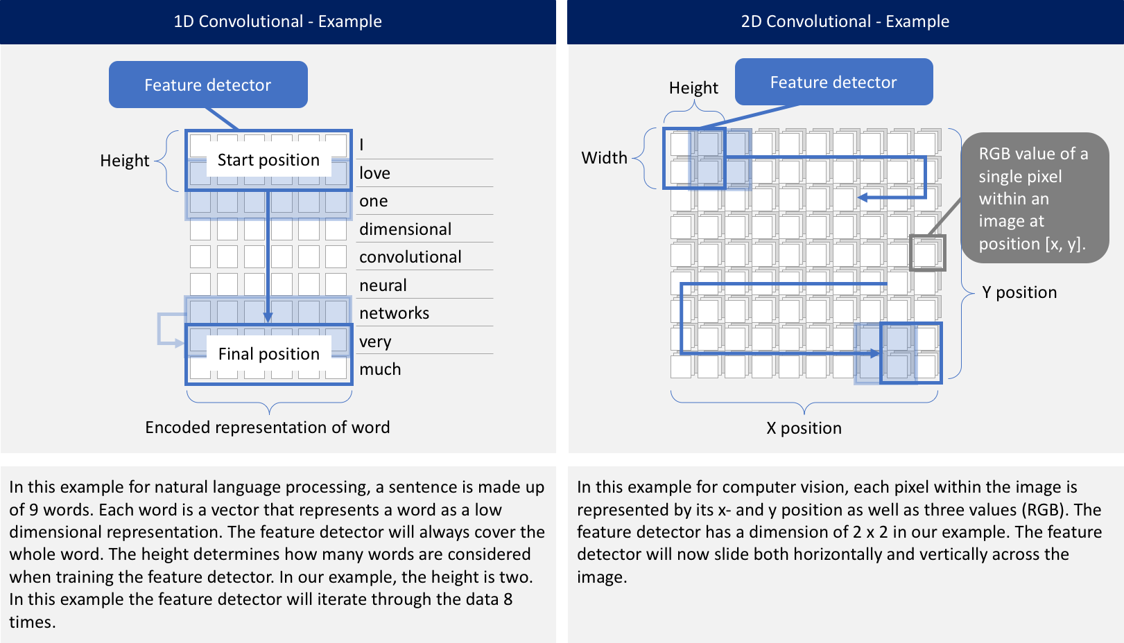
What is the Difference Between a 1D CNN and a 2D CNN?
無論是1D,2D還是3D。 關鍵區別在於輸入數據的維度以及特徵檢測器(或過濾器)如何在數據中滑動:
Problem Statement
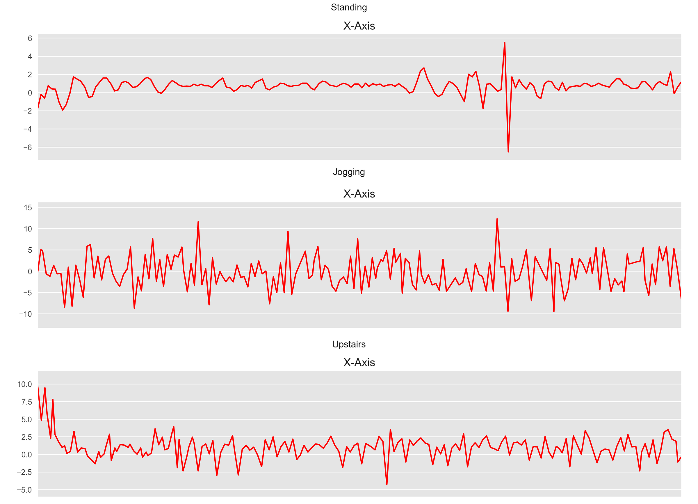
在本文中,我們將重點關注來自用戶腰部攜帶的智能手機其時間切片加速計傳感器數據。 基於x,y和z軸的加速度計數據,1D CNN應預測用戶正在執行的活動類型(例如“行走”,“慢跑”或“站立”)。 您可以在此處和此處的其他兩篇文章中找到更多資訊。
https://towardsdatascience.com/human-activity-recognition-har-tutorial-with-keras-and-core-ml-part-1-8c05e365dfa0
https://towardsdatascience.com/human-activity-recognition-har-tutorial-with-keras-and-core-ml-part-2-857104583d94
對於各種活動,數據的每個時間間隔看起來都類似於此。
How to Construct a 1D CNN in Python?
有許多標準CNN模組可供選擇。 我選擇了Keras網站上描述的其中一個模型並對其進行了微調,以吻合上述問題。 下圖提供了高級概述的構建模型。 將進一步解釋每一層。
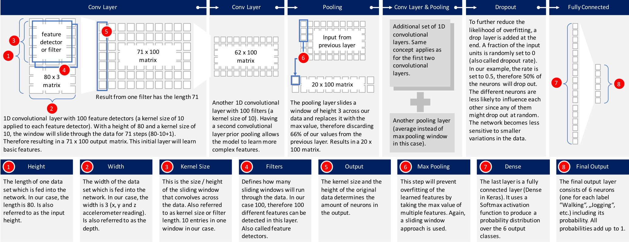
但是,讓我們首先看一下Python代碼,以構建這個模型:
執行此代碼將導致以下深度神經網絡:
讓我們深入了解每一層,看看發生了什麼:
1. 輸入數據:數據已經過前處理,每個數據記錄包含80個時間片段(數據以20 Hz採樣率記錄,因此每個時間間隔覆蓋4秒的加速度計讀數)。 在每個時間間隔內,存儲x軸,y軸和z軸的三個加速度計值。 這導致80×3矩陣。 由於我通常在iOS中使用神經網絡,因此必須將數據作為長度為240的扁平化向量傳遞到神經網絡中。網絡中的第一層必須將其重新整形為80 x 3的原始形狀。
2. 第一個1D CNN層:第一層定義高度為10的過濾器(或稱為特徵檢測器)(也稱為內核大小)。 僅定義一個過濾器將允許神經網絡去學習第一層中的單特徵。 這可能還不夠,因此我們將定義100個過濾器。 這允許我們在網絡的第一層上訓練100個不同的特徵。 第一神經網絡層的輸出是71×100神經元矩陣。 輸出矩陣的每列保持一個單個濾波器的權重。 使用定義的內核大小並考慮輸入矩陣的長度,每個過濾器將包含71個權重。
3. 第二個1D CNN層:來自第一個CNN的結果將被饋送到第二個CNN層。 我們將再次定義100個不同的過濾器,以便在此級別上進行訓練。 遵循與第一層相同的邏輯,輸出矩陣的大小為62 x 100。
4. 最大池化層:通常在CNN層之後使用池化層,以降低輸出的複雜性並防止數據過度擬合。 在我們的例子中,我們選擇了三個大小。 這意味著該層的輸出矩陣的大小僅為輸入矩陣的三分之一。
5. 第三和第四1D CNN層:遵循另一序列的1D CNN層以便學習更高階特徵。 這兩層之後的輸出矩陣是2×160矩陣。
6. 平均池化層:再一個池化層,以進一步避免過度擬合。這次不是取最大值,而是神經網絡中兩個權重的平均值。輸出矩陣的大小為1 x 160個神經元。每個特徵檢測器在該層上的神經網絡中僅剩餘一個權重。
7. Dropout層:Dropout層將隨機分配0個權重給網絡中的神經元。由於我們選擇0.5的比率,50%的神經元將獲得零權重。通過此操作,網絡對較小的數據變化做出反應變得不那麼敏感。因此,它應該進一步提高我們對未知類別新資料的準確性。該層的輸出仍然是1 x 160的神經元矩陣。
8. 具有Softmax激活的完全連接層:最後一層將高度160的向量減少到六的向量,因為我們有六個類我們想要預測(“慢跑”,“坐著”,“行走”,“站立”,“樓上樓下”)。這種減少是透過另一個矩陣乘法完成的。 Softmax用作激活函數。它強制神經網絡的所有六個輸出總和為一。因此,輸出值將代表六個類別中每個類別的概率。
Training and Testing the Neural Network
下面是用於訓練模型的Python代碼,批量大小為400,訓練和驗證分為80到20。
該模型對於訓練數據達到97%的準確度。
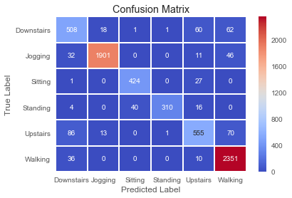
針對測試數據運行它可以發現92%的準確率。
考慮到我們使用標準1D CNN模型之一,這是一個很好的數字。 我們的模型在精確度,召回率和f1-score方面也得分很高。
以下簡要回顧一下這些分數的含義:
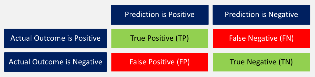
1. 準確度:正確預測結果與所有預測總和之間的比率。 ((TP + TN) / (TP + TN + FP + FN))
2. 精確度:當模型預測為positive時,是不是? 所有true positives除以所有positive預測。 (TP / (TP + FP))
3. 召回率:該模型在所有可能的positives中確定了多少positives? true positives除以所有實際positives。 (TP / (TP + FN))
4. F1-score:這是精確度和召回率的加權平均值。 (2 x召回率x精度/(召回率+精確度))
針對測試數據的相關混淆矩陣如下所示。
Summary
在本文中,您已經看到了一個範例,說明如何使用1D CNN來訓練網絡,以根據智能手機的一組給定加速度計數據預測用戶行為。 完整的Python代碼可以在github上找到。
參考
https://blog.goodaudience.com/introduction-to-1d-convolutional-neural-networks-in-keras-for-time-sequences-3a7ff801a2cf?fbclid=IwAR0B11L3DXkTHqheCSYpG1SetABlWcREFsnLQf5tSdVbFtcVkkjr9zCdngw
許多文章都集中在二維卷積神經網絡上。 它們特別用於圖像識別問題。 1D CNN在某種程度上被隱匿,例如, 用於自然語言處理(NLP)。 很少有文章提供關於如何構建1D CNN的逐步指令解釋,以及您可能面臨的其他機器學習問題。 本文試圖彌合這一差距。
When to Apply a 1D CNN?
CNN非常適合識別數據中的簡單模式,然後用在更高階層中形成更複雜的模式。 當您希望從整個數據集較短(固定長度)段落中獲得有趣的特徵並且該段落中的特徵的位置不具有高度相關性時,1D CNN是非常有效的。
這很適用於傳感器數據的時間序列分析(例如陀螺儀或加速度計數據)。 它還適用於在固定長度週期內(例如音頻信號)分析任何類型的信號數據。 另一個應用是NLP(雖然這裡LSTM網絡更有前景,因為鄰近的單詞在訓練模式下可能並不是良好的指標)。
What is the Difference Between a 1D CNN and a 2D CNN?
無論是1D,2D還是3D。 關鍵區別在於輸入數據的維度以及特徵檢測器(或過濾器)如何在數據中滑動:
Problem Statement
在本文中,我們將重點關注來自用戶腰部攜帶的智能手機其時間切片加速計傳感器數據。 基於x,y和z軸的加速度計數據,1D CNN應預測用戶正在執行的活動類型(例如“行走”,“慢跑”或“站立”)。 您可以在此處和此處的其他兩篇文章中找到更多資訊。
https://towardsdatascience.com/human-activity-recognition-har-tutorial-with-keras-and-core-ml-part-1-8c05e365dfa0
https://towardsdatascience.com/human-activity-recognition-har-tutorial-with-keras-and-core-ml-part-2-857104583d94
對於各種活動,數據的每個時間間隔看起來都類似於此。
How to Construct a 1D CNN in Python?
有許多標準CNN模組可供選擇。 我選擇了Keras網站上描述的其中一個模型並對其進行了微調,以吻合上述問題。 下圖提供了高級概述的構建模型。 將進一步解釋每一層。
但是,讓我們首先看一下Python代碼,以構建這個模型:
model_m = Sequential()
model_m.add(Reshape((TIME_PERIODS, num_sensors), input_shape=(input_shape,)))
model_m.add(Conv1D(100, 10, activation='relu', input_shape=(TIME_PERIODS, num_sensors)))
model_m.add(Conv1D(100, 10, activation='relu'))
model_m.add(MaxPooling1D(3))
model_m.add(Conv1D(160, 10, activation='relu'))
model_m.add(Conv1D(160, 10, activation='relu'))
model_m.add(GlobalAveragePooling1D())
model_m.add(Dropout(0.5))
model_m.add(Dense(num_classes, activation='softmax'))
print(model_m.summary())
執行此代碼將導致以下深度神經網絡:
_________________________________________________________________
Layer (type)                 Output Shape              Param #
=================================================================
reshape_45 (Reshape)         (None, 80, 3)             0
_________________________________________________________________
conv1d_145 (Conv1D)          (None, 71, 100)           3100
_________________________________________________________________
conv1d_146 (Conv1D)          (None, 62, 100)           100100
_________________________________________________________________
max_pooling1d_39 (MaxPooling (None, 20, 100)           0
_________________________________________________________________
conv1d_147 (Conv1D)          (None, 11, 160)           160160
_________________________________________________________________
conv1d_148 (Conv1D)          (None, 2, 160)            256160
_________________________________________________________________
global_average_pooling1d_29  (None, 160)               0
_________________________________________________________________
dropout_29 (Dropout)         (None, 160)               0
_________________________________________________________________
dense_29 (Dense)             (None, 6)                 966
=================================================================
Total params: 520,486
Trainable params: 520,486
Non-trainable params: 0
_________________________________________________________________
None
讓我們深入了解每一層,看看發生了什麼:
1. 輸入數據:數據已經過前處理,每個數據記錄包含80個時間片段(數據以20 Hz採樣率記錄,因此每個時間間隔覆蓋4秒的加速度計讀數)。 在每個時間間隔內,存儲x軸,y軸和z軸的三個加速度計值。 這導致80×3矩陣。 由於我通常在iOS中使用神經網絡,因此必須將數據作為長度為240的扁平化向量傳遞到神經網絡中。網絡中的第一層必須將其重新整形為80 x 3的原始形狀。
3. 第二個1D CNN層:來自第一個CNN的結果將被饋送到第二個CNN層。 我們將再次定義100個不同的過濾器,以便在此級別上進行訓練。 遵循與第一層相同的邏輯,輸出矩陣的大小為62 x 100。
4. 最大池化層:通常在CNN層之後使用池化層,以降低輸出的複雜性並防止數據過度擬合。 在我們的例子中,我們選擇了三個大小。 這意味著該層的輸出矩陣的大小僅為輸入矩陣的三分之一。
5. 第三和第四1D CNN層:遵循另一序列的1D CNN層以便學習更高階特徵。 這兩層之後的輸出矩陣是2×160矩陣。
6. 平均池化層:再一個池化層,以進一步避免過度擬合。這次不是取最大值,而是神經網絡中兩個權重的平均值。輸出矩陣的大小為1 x 160個神經元。每個特徵檢測器在該層上的神經網絡中僅剩餘一個權重。
7. Dropout層:Dropout層將隨機分配0個權重給網絡中的神經元。由於我們選擇0.5的比率,50%的神經元將獲得零權重。通過此操作,網絡對較小的數據變化做出反應變得不那麼敏感。因此,它應該進一步提高我們對未知類別新資料的準確性。該層的輸出仍然是1 x 160的神經元矩陣。
8. 具有Softmax激活的完全連接層:最後一層將高度160的向量減少到六的向量,因為我們有六個類我們想要預測(“慢跑”,“坐著”,“行走”,“站立”,“樓上樓下”)。這種減少是透過另一個矩陣乘法完成的。 Softmax用作激活函數。它強制神經網絡的所有六個輸出總和為一。因此,輸出值將代表六個類別中每個類別的概率。
Training and Testing the Neural Network
下面是用於訓練模型的Python代碼,批量大小為400,訓練和驗證分為80到20。
callbacks_list = [
    keras.callbacks.ModelCheckpoint(
        filepath='best_model.{epoch:02d}-{val_loss:.2f}.h5',
        monitor='val_loss', save_best_only=True),
    keras.callbacks.EarlyStopping(monitor='acc', patience=1)
]

model_m.compile(loss='categorical_crossentropy',
                optimizer='adam', metrics=['accuracy'])

BATCH_SIZE = 400
EPOCHS = 50

history = model_m.fit(x_train,
                      y_train,
                      batch_size=BATCH_SIZE,
                      epochs=EPOCHS,
                      callbacks=callbacks_list,
                      validation_split=0.2,
                      verbose=1)
該模型對於訓練數據達到97%的準確度。
...
Epoch 9/50
16694/16694 [==============================] - 16s 973us/step - loss: 0.0975 - acc: 0.9683 - val_loss: 0.7468 - val_acc: 0.8031
Epoch 10/50
16694/16694 [==============================] - 17s 989us/step - loss: 0.0917 - acc: 0.9715 - val_loss: 0.7215 - val_acc: 0.8064
Epoch 11/50
16694/16694 [==============================] - 17s 1ms/step - loss: 0.0877 - acc: 0.9716 - val_loss: 0.7233 - val_acc: 0.8040
Epoch 12/50
16694/16694 [==============================] - 17s 1ms/step - loss: 0.0659 - acc: 0.9802 - val_loss: 0.7064 - val_acc: 0.8347
Epoch 13/50
16694/16694 [==============================] - 17s 1ms/step - loss: 0.0626 - acc: 0.9799 - val_loss: 0.7219 - val_acc: 0.8107
針對測試數據運行它可以發現92%的準確率。
Accuracy on test data: 0.92
Loss on test data: 0.39
考慮到我們使用標準1D CNN模型之一,這是一個很好的數字。 我們的模型在精確度,召回率和f1-score方面也得分很高。
precision recall f1-score support
0                 0.76      0.78      0.77       650
1                 0.98      0.96      0.97      1990
2                 0.91      0.94      0.92       452
3                 0.99      0.84      0.91       370
4                 0.82      0.77      0.79       725
5                 0.93      0.98      0.95      2397
avg / total 0.92 0.92 0.92 6584
以下簡要回顧一下這些分數的含義:
1. 準確度:正確預測結果與所有預測總和之間的比率。 ((TP + TN) / (TP + TN + FP + FN))
2. 精確度:當模型預測為positive時,是不是? 所有true positives除以所有positive預測。 (TP / (TP + FP))
3. 召回率:該模型在所有可能的positives中確定了多少positives? true positives除以所有實際positives。 (TP / (TP + FN))
4. F1-score:這是精確度和召回率的加權平均值。 (2 x召回率x精度/(召回率+精確度))
針對測試數據的相關混淆矩陣如下所示。
Summary
在本文中,您已經看到了一個範例,說明如何使用1D CNN來訓練網絡,以根據智能手機的一組給定加速度計數據預測用戶行為。 完整的Python代碼可以在github上找到。
參考
https://blog.goodaudience.com/introduction-to-1d-convolutional-neural-networks-in-keras-for-time-sequences-3a7ff801a2cf?fbclid=IwAR0B11L3DXkTHqheCSYpG1SetABlWcREFsnLQf5tSdVbFtcVkkjr9zCdngw
2019年7月27日 星期六
How to implement a neural network - gradient descent
這可能會給你帶來驚喜:神經網絡並不複雜! 術語“神經網絡”被廣泛用作流行語,但實際上它們通常比人們想像的要簡單得多。
本文僅供初學者使用,並假設ZERO具有機器學習的先驗知識。 我們將理解神經網絡如何在Python中從頭開始實現。
讓我們開始吧!
本文僅供初學者使用,並假設ZERO具有機器學習的先驗知識。 我們將理解神經網絡如何在Python中從頭開始實現。
讓我們開始吧!
2019年7月26日 星期五
What Is K means clustering Algorithm in Python
K表示聚類是一種無監督學習演算法,它根據最近的平均值將n個對象劃分為k個clusters。 該模組突顯了K-means演算法,K的使用意味著clustering,在本模組的最後,我們將藉助Iris數據集構建K means clustering模型。
Data Science K-means Clustering – In-depth Tutorial with Example
最流行的機器學習算法之一是K-means clustering。 它是一種無監督學習算法,意味著它用於未標記的數據集。 想像一下,你有幾個點分佈在一個n維空間。 為了根據它們的相似性對這些數據進行分類,您將使用K-means clustering演算法。 在本文中,我們將詳細介紹此演算法。 然後,我們將討論基本Python函式庫可用於實現此演算法。
K-means clustering演算法是一種無監督技術,按照它們的相似性順序對數據進行分組。 然後,我們在有k-clusters數據中找到模式。 這些集群基本上是基於它們的相似性聚合的數據點。 讓我們開始K-means Clustering教學,簡要介紹一下群集。

What is Clustering?
想像一下,你有一組巧克力和甘草糖。 你需要將兩個食物分開。 直觀地,您可以根據它們的外觀將它們分開。 將對象基於它們各自的特徵分成團的過程稱為集群(Clustering)。
集群用於各種領域,如圖像識別,模式分析,醫學信息學,基因組學,數據壓縮等。它是機器學習中無監督學習算法的一部分。 這是因為存在的數據點沒有標記,並且沒有輸入和輸出的顯式映射。 因此,基於內部存在的模式,發生集群。
What is K-means Clustering?
根據K-means clustering的形式定義 - K-means clustering是一種迭代演算法,它將包含n個值的一組數據劃分為k個子組。 n值中的每一個都屬於具有最接近平均值的k cluster。
這意味著給定一組對象,我們將該組分成幾個子組。 這些子組基於它們的相似性以及子組中每個數據點的距離與它們的質心的平均值所形成。 K-means clustering是無監督學習演算法裡最流行的形式。 它易於理解和實施。
K-means clustering的目的是最小化歐幾里德距離,也就是每個點與cluster質心的距離。 這稱為intra-cluster variance,可以使用以下平方誤差函數進行最小化 -

其中J是cluster質心的目標函數。 K是cluster的數量,n是個案的數量。 C是質心數,j是cluster數。 X是給定的數據點,我們必須決定X與質心的歐幾里德距離。 讓我們看一下K-means clustering的演算法 -
(i) 首先,我們隨機初始化並選擇k點。 這些k點是工具。
(ii) 我們使用歐幾里德距離來找到最接近cluster中心的數據點。
(iii) 然後我們計算cluster中所有點的平均值來找到其質心。
(iv) 我們迭代地重複步驟1,2和3,直到將所有點分配給它們各自的clusters。
K-Means是一種非層次clustering方法。
K-Means in Action
在本節中,我們將利用Python函式庫產生隨機數據來執行K-means。
首先,我們導入基本Python庫來執行k-means演算法 -

從上圖中,我們觀察到在兩個clusters中劃分了大約200個數據點,其中每個cluster包含100個數據點。
在繪製了兩個clusters之後,我們繼續執行我們的k-means學習演算法來為我們的cluster建立質心。 我們啟動k,它代表隨機值為3的集群。

在上面的可視化中,我們獲得了兩個clusters的質心。 現在,我們將測試我們的模型。 在測試階段,首先我們將顯示兩個標籤(0,1)分佈代表兩個clusters。
現在,我們預測一個給定數據點位於二維空間中位置(4,5)的cluster。
Applications of K-Means Clustering Algorithm
(i) K-means演算法用於商業領域來識別用戶進行購買部分。 它還用於網站上的群集活動。
(ii) 它被用於破壞性資料壓縮技術(lossy image compression technique)的一種形式。 在圖像壓縮中,K-means用於群集圖像的像素,從而減小其整體尺寸。
(iii) 它也用於文件分群來查找相關文檔。
(iv) K-means用於保險和欺詐檢測領域。 根據以前的歷史數據,可以根據欺詐模式的集群接近程度來分群欺詐行為和索賠。
(v) 它還用於根據聲音的相似模式對聲音進行分類,並隔離語音中的瑕疵。
(vi) K-means clustering用於通聯記錄(Call Detail Record, CDR)分析。 它可以根據當天的通話量和場所的人口統計信息深入了解客戶需求。
Summary
因此,在這個K-means clustering教學中,我們了解了它的基礎知識。 我們理解它的定義和使用的演算法。 我們還使用Python函式庫進行代碼。 最後,我們經歷了K-means clustering的實際應用。 作為數據科學家,了解這種clustering演算法至關重要。 因為它教你處理未標記的數據,所以對於任何嶄露頭角的數據科學家來說,它都是必備的技能。
K-means是一種機器學習演算法,它構成了一個更大的數據操作池的一部分,稱為數據科學(Data Science)。 現在是探索數據科學一切的最佳時機。
參考
https://data-flair.training/blogs/k-means-clustering-tutorial/?fbclid=IwAR0rba-RVvye4VQBtCi8z9I-8mpsvi6-VBpOoBz1sfmhDieSFMbG5Cx-Vhg
K-means clustering演算法是一種無監督技術,按照它們的相似性順序對數據進行分組。 然後,我們在有k-clusters數據中找到模式。 這些集群基本上是基於它們的相似性聚合的數據點。 讓我們開始K-means Clustering教學,簡要介紹一下群集。
What is Clustering?
想像一下,你有一組巧克力和甘草糖。 你需要將兩個食物分開。 直觀地,您可以根據它們的外觀將它們分開。 將對象基於它們各自的特徵分成團的過程稱為集群(Clustering)。
集群用於各種領域,如圖像識別,模式分析,醫學信息學,基因組學,數據壓縮等。它是機器學習中無監督學習算法的一部分。 這是因為存在的數據點沒有標記,並且沒有輸入和輸出的顯式映射。 因此,基於內部存在的模式,發生集群。
What is K-means Clustering?
根據K-means clustering的形式定義 - K-means clustering是一種迭代演算法,它將包含n個值的一組數據劃分為k個子組。 n值中的每一個都屬於具有最接近平均值的k cluster。
這意味著給定一組對象,我們將該組分成幾個子組。 這些子組基於它們的相似性以及子組中每個數據點的距離與它們的質心的平均值所形成。 K-means clustering是無監督學習演算法裡最流行的形式。 它易於理解和實施。
K-means clustering的目的是最小化歐幾里德距離,也就是每個點與cluster質心的距離。 這稱為intra-cluster variance,可以使用以下平方誤差函數進行最小化 -
其中J是cluster質心的目標函數。 K是cluster的數量,n是個案的數量。 C是質心數,j是cluster數。 X是給定的數據點,我們必須決定X與質心的歐幾里德距離。 讓我們看一下K-means clustering的演算法 -
(i) 首先,我們隨機初始化並選擇k點。 這些k點是工具。
(ii) 我們使用歐幾里德距離來找到最接近cluster中心的數據點。
(iii) 然後我們計算cluster中所有點的平均值來找到其質心。
(iv) 我們迭代地重複步驟1,2和3,直到將所有點分配給它們各自的clusters。
K-Means是一種非層次clustering方法。
K-Means in Action
在本節中,我們將利用Python函式庫產生隨機數據來執行K-means。
首先,我們導入基本Python庫來執行k-means演算法 -
- import numpy as np
- import pandas as pd
- import matplotlib.pyplot as plt
- from sklearn.cluster import KMeans
- x = -2 * np.random.rand(200,2)
- x0 = 1 + 2 * np.random.rand(100,2)
- x[100:200, :] = x0
- plt.scatter(x[ : , 0], x[ :, 1], s = 25, color='r')
- plt.grid()
從上圖中,我們觀察到在兩個clusters中劃分了大約200個數據點,其中每個cluster包含100個數據點。
在繪製了兩個clusters之後,我們繼續執行我們的k-means學習演算法來為我們的cluster建立質心。 我們啟動k,它代表隨機值為3的集群。
- Kmean = KMeans(n_clusters=3)
- Kmean.fit(x)
- Kmean.cluster_centers_
- plt.scatter(2.03078996, 2.05446538, s=100, color='green')
- plt.show()
在上面的可視化中,我們獲得了兩個clusters的質心。 現在,我們將測試我們的模型。 在測試階段,首先我們將顯示兩個標籤(0,1)分佈代表兩個clusters。
- Kmean.labels_
現在,我們預測一個給定數據點位於二維空間中位置(4,5)的cluster。
- sample_test=np.array([4.0,5.0])
- second_test=sample_test.reshape(1, -1)
- Kmean.predict(second_test)
Applications of K-Means Clustering Algorithm
(i) K-means演算法用於商業領域來識別用戶進行購買部分。 它還用於網站上的群集活動。
(ii) 它被用於破壞性資料壓縮技術(lossy image compression technique)的一種形式。 在圖像壓縮中,K-means用於群集圖像的像素,從而減小其整體尺寸。
(iii) 它也用於文件分群來查找相關文檔。
(iv) K-means用於保險和欺詐檢測領域。 根據以前的歷史數據,可以根據欺詐模式的集群接近程度來分群欺詐行為和索賠。
(v) 它還用於根據聲音的相似模式對聲音進行分類,並隔離語音中的瑕疵。
(vi) K-means clustering用於通聯記錄(Call Detail Record, CDR)分析。 它可以根據當天的通話量和場所的人口統計信息深入了解客戶需求。
Summary
因此,在這個K-means clustering教學中,我們了解了它的基礎知識。 我們理解它的定義和使用的演算法。 我們還使用Python函式庫進行代碼。 最後,我們經歷了K-means clustering的實際應用。 作為數據科學家,了解這種clustering演算法至關重要。 因為它教你處理未標記的數據,所以對於任何嶄露頭角的數據科學家來說,它都是必備的技能。
K-means是一種機器學習演算法,它構成了一個更大的數據操作池的一部分,稱為數據科學(Data Science)。 現在是探索數據科學一切的最佳時機。
參考
https://data-flair.training/blogs/k-means-clustering-tutorial/?fbclid=IwAR0rba-RVvye4VQBtCi8z9I-8mpsvi6-VBpOoBz1sfmhDieSFMbG5Cx-Vhg
Covariance and Correlation
共變異數(Covariance)和相關性(Correlation)非常有助於理解兩個連續變量之間的關係。 共變異數指出兩個變量是在相同方向(正變異數)還是在相反方向(負變異數)上變化。 變異數值沒有意義,只有符號才有用。 而相關性解釋了一個變量的變化導致第二個變量的比例變化有多大。 相關性在-1到+1之間變化。 如果相關值為0則表示變量之間沒有線性關係,但可能存在其他函數關係。
讓我們詳細了解這些術語:
讓我們詳細了解這些術語:
2019年7月25日 星期四
2019年7月24日 星期三

2019年7月20日 星期六
2019年7月19日 星期五
2019年7月17日 星期三
2019年7月16日 星期二
2019年7月10日 星期三
常用的Pandas應用在機器學習
1. csv
(i) df = ps.read_csv("./input/ecoli.csv", delim_whitespace=True)
(ii) df = pd.read_csv(filepath, names=['sentence', 'label'], sep='\t')
(ii) url = 'https://archive.ics.uci.edu/ml/machine-learning-databases/molecular-biology/promoter-gene-sequences/promoters.data'
names = ['Class', 'id', 'Sequence']
df = pd.read_csv(url, names = names)
2. assign column
pd.columns = ['seq_name', 'mcg', 'gvh', 'lip', 'chg', 'aac', 'alm1', 'alm2', 'site']
3. drop
(i) df = pd.drop('seq_name', axis=1)
(ii) df = pd.drop(columns=['seq_name'])
4. replace
pd.replace(('cp', 'im', 'pp', 'imU', 'om', 'omL', 'imL', 'imS'),(1,2,3,4,5,6,7,8), inplace=True)
5. Statistical Description
pd.describe()
6. shape
pd.shape
7. type
pd.dtypes
8. correlation coefficient
pd.corr(method='pearson')
9. value (type=numpy)
df = pd.values
10. loc
df = pd.loc[:, 'Class']
11. transpose
df = pd.transpose()
12. rename
(i) pd.rename(columns = {57: 'Class'}, inplace = True)
(ii) sequences.rename("sequences")
13. value_counts()
df[name].value_counts()
14. one-hot encoder
df = pd.get_dummies(df)
15. head
pd.head()
16. txt
df = pd.read_table('chimp_data.txt')
17. apply
df['words'] = pd.apply(lambda x: getKmers(x['sequence']), axis=1)
18. merge
df = pd.read_csv('./input/pdb_data_no_dups.csv').merge(pd.read_csv('./input/pdb_data_seq.csv'), how='inner', on='structureId')
19. reset_index
pd.reset_index()
sequences.reset_index(drop=True, inplace=True)
20. dropna
sequences=df[0].dropna()
21. concat
df = pd.concat([df1,df2,df3], axis=1)
22. modify column value
pd['label']='1'
23. df[condiction]
df_yelp = df[df['source'] == 'yelp']
24. unique
pd.Series([2, 1, 3, 3], name='A').unique()
df['source'].unique()
2019年7月9日 星期二
Classifying DNA Sequences
本文中將使用馬爾可夫模型,K-最近鄰(KNN)算法,支持向量機和其他常見分類器來分析短大腸桿菌DNA序列,從而探索生物信息學的世界。 該項目將使用來自UCI Machine Learning Repository的數據集,該數據集具有106個DNA序列,每個具有57個連續核苷酸(“鹼基對”)。
將會學到如何:
1. 從UCI存儲庫導入數據
2. 將文本輸入轉換為數值型資料
3. 構建和訓練分類演算法
4. 比較和對比分類演算法
Step 1: Importing the Dataset
以下代碼單元將導入重要的函式庫,並從UCI存儲庫導入數據集作為Pandas DataFrame。


Step 2: Preprocessing the Dataset
數據不是可用的形式; 因此,我們需要在使用它來訓練我們的演算法之前對其進行處理。


print(X.shape)
print(type(X))
print(type(X[0]))
print(type(X[0][0]))
(106, 228)
<class 'numpy.ndarray'>
<class 'numpy.ndarray'>
<class 'numpy.uint8'>
Step 3: Training and Testing the Classification Algorithms
現在我們已經預處理了數據並構建了我們的訓練和測試數據集,我們可以開始部署不同的分類演算法。 測試多個模型相對容易; 因此,我們將比較和對比十種不同演算法的性能。

參考
https://www.kaggle.com/bulentsiyah/dna-classification-code
將會學到如何:
1. 從UCI存儲庫導入數據
2. 將文本輸入轉換為數值型資料
3. 構建和訓練分類演算法
4. 比較和對比分類演算法
Step 1: Importing the Dataset
以下代碼單元將導入重要的函式庫,並從UCI存儲庫導入數據集作為Pandas DataFrame。
# To make sure all of the correct libraries are installed, import each module and print the version number

import sys
import numpy
import sklearn
import pandas

print('Python: {}'.format(sys.version))
print('Numpy: {}'.format(numpy.__version__))
print('Sklearn: {}'.format(sklearn.__version__))
print('Pandas: {}'.format(pandas.__version__))

# Import, change module names
import numpy as np
import pandas as pd

# import the uci Molecular Biology (Promoter Gene Sequences) Data Set
url = 'https://archive.ics.uci.edu/ml/machine-learning-databases/molecular-biology/promoter-gene-sequences/promoters.data'
names = ['Class', 'id', 'Sequence']
data = pd.read_csv(url, names = names)
print(data.iloc[0])

Step 2: Preprocessing the Dataset
數據不是可用的形式; 因此,我們需要在使用它來訓練我們的演算法之前對其進行處理。
# Building our Dataset by creating a custom Pandas DataFrame
# Each column in a DataFrame is called a Series. Lets start by making a series for each column.

classes = data.loc[:, 'Class']
print(classes[:5])

# generate list of DNA sequences
sequences = list(data.loc[:, 'Sequence'])
dataset = {}

# loop through sequences and split into individual nucleotides
for i, seq in enumerate(sequences):

    # split into nucleotides, remove tab characters
    nucleotides = list(seq)
    nucleotides = [x for x in nucleotides if x != '\t']

    # append class assignment
    nucleotides.append(classes[i])

    # add to dataset
    dataset[i] = nucleotides

print(dataset[0])

# turn dataset into pandas DataFrame
dframe = pd.DataFrame(dataset)
print(dframe)

# transpose the DataFrame
df = dframe.transpose()
print(df.iloc[:5])

# for clarity, lets rename the last dataframe column to class
df.rename(columns = {57: 'Class'}, inplace = True)
print(df.iloc[:5])

# looks good! Let's start to familiarize ourselves with the dataset so we can pick the most suitable
# algorithms for this data

df.describe()

# desribe does not tell us enough information since the attributes are text. Lets record value counts for each sequence
series = []
for name in df.columns:
    series.append(df[name].value_counts())

info = pd.DataFrame(series)
details = info.transpose()
print(details)

# Unfortunately, we can't run machine learning algorithms on the data in 'String' formats. As a result, we need to switch
# it to numerical data. This can easily be accomplished using the pd.get_dummies() function
numerical_df = pd.get_dummies(df)
numerical_df.iloc[:5]

# We don't need both class columns.  Lets drop one then rename the other to simply 'Class'.
df = numerical_df.drop(columns=['57_-'])

df.rename(columns = {'57_+': 'Class'}, inplace = True)
print(df.iloc[:5])

# Use the model_selection module to separate training and testing datasets
from sklearn import model_selection

# Create X and Y datasets for training
X = np.array(df.drop(['Class'], 1))
y = np.array(df['Class'])

# define seed for reproducibility
seed = 1

# split data into training and testing datasets
X_train, X_test, y_train, y_test = model_selection.train_test_split(X, y, test_size=0.25, random_state=seed)
print(X.shape)
print(type(X))
print(type(X[0]))
print(type(X[0][0]))
(106, 228)
<class 'numpy.ndarray'>
<class 'numpy.ndarray'>
<class 'numpy.uint8'>
Step 3: Training and Testing the Classification Algorithms
現在我們已經預處理了數據並構建了我們的訓練和測試數據集,我們可以開始部署不同的分類演算法。 測試多個模型相對容易; 因此,我們將比較和對比十種不同演算法的性能。
# Now that we have our dataset, we can start building algorithms! We'll need to import each algorithm we plan on using
# from sklearn.  We also need to import some performance metrics, such as accuracy_score and classification_report.

from sklearn.neighbors import KNeighborsClassifier
from sklearn.neural_network import MLPClassifier
from sklearn.gaussian_process import GaussianProcessClassifier
from sklearn.gaussian_process.kernels import RBF
from sklearn.tree import DecisionTreeClassifier
from sklearn.ensemble import RandomForestClassifier, AdaBoostClassifier
from sklearn.naive_bayes import GaussianNB
from sklearn.svm import SVC
from sklearn.metrics import classification_report, accuracy_score

# define scoring method
scoring = 'accuracy'

# Define models to train
names = ["Nearest Neighbors", "Gaussian Process",
         "Decision Tree", "Random Forest", "Neural Net", "AdaBoost",
         "Naive Bayes", "SVM Linear", "SVM RBF", "SVM Sigmoid"]

classifiers = [
    KNeighborsClassifier(n_neighbors = 3),
    GaussianProcessClassifier(1.0 * RBF(1.0)),
    DecisionTreeClassifier(max_depth=5),
    RandomForestClassifier(max_depth=5, n_estimators=10, max_features=1),
    MLPClassifier(alpha=1e-5),
    AdaBoostClassifier(),
    GaussianNB(),
    SVC(kernel = 'linear', gamma='auto'),
SVC(kernel = 'rbf', gamma='auto'),
SVC(kernel = 'sigmoid', gamma='auto')
]
models = zip(names, classifiers)

# evaluate each model in turn
results = []
names = []

for name, model in models:
    kfold = model_selection.KFold(n_splits=10, random_state = seed)
    cv_results = model_selection.cross_val_score(model, X_train, y_train, cv=kfold, scoring=scoring)
    results.append(cv_results)
    names.append(name)
    msg = "%s: %f (%f)" % (name, cv_results.mean(), cv_results.std())
    print(msg)
    model.fit(X_train, y_train)
    predictions = model.predict(X_test)
    print('Test-- ',name,': ',accuracy_score(y_test, predictions))
    print()
    print(classification_report(y_test, predictions))

參考
https://www.kaggle.com/bulentsiyah/dna-classification-code
訂閱:
文章 (Atom)